


My previous article in the April issue of Pumps & Systems (read it here) on the use of automated data acquisition systems focused on testing two pumps individually to compare the pumps’ actual performance to the predicted OEM curve for a new pump.
The system (PREMS-2A), operating continuously, logs flow, power, pressure, vibration, temperature and other data parameters. Software translates that data into a “pump curves language,” displaying the resultant performance live on the computer screen remotely and continually. As we saw, the actual performance displayed reduced performance, resulting in wasted energy.
The clusters of data showed the main flow regions the two pumps operated during the testing. However, on the same plot, there were clusters of data with pump head being oddly out-of-line with the rest of the tracked data. The parting quiz to our readers was to explain the reason why a pump head at certain times was considerably greater than the rest of the logged displayed data.
I received feedback from several people on this question, including Lee Ruiz of Oceanside, California:
Dr. Nelik,
Thanks for your articles. In your April field efficiency case study, it appears that figure 4 (April-17 P&S) is a combination of pump 1 performance in addition to the parallel operation of 1 & 2 operating together.
Right on, Lee! That is exactly what the PREMS-2A system picked up: a two-pump operation, resulting in higher total head but not necessarily a proportional increase in flow. This means our system is “friction-dominated,” with elevation head being negligible (see Figure 1).
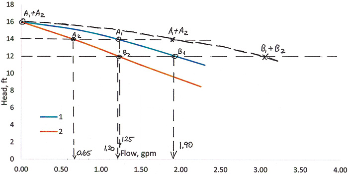 Figure 1. Combined (two pumps) operation explanation (Courtesy of the author)
To analyze this, we first replot the head-capacity curves for each pump and then add the flow at same heads, picking several (three in this case) horizontal head lines to interest the curves. At 14 feet of head, for example, a “stronger” pump 1 shows 1.25 gpm, while a “weaker” pump 2 generates only 0.65 gpm, thus a 1.9 gpm total, as shown by points A1 plus A2. Similarly, at 12 feed of head, pumps produce 1.2 gpm plus 1.9 gpm, a 3.1 gpm total (B1+B2).
The PREMS-2A system did all that automatically and online for us, as shown on the system screen continually, but Figure 1 helps us dissect the result and explain what happens when pumps operate in parallel.
Note that construction of the resultant two-pump curve does not require each pump to be identical. In our example, shut-off heads for each pump are the same, but in general that is not required for the construction of the resultant curve. However, the actual operation of the significantly dissimilar pumps (hydraulically) is not recommended (the weaker one will be “pushed out,” but the resultant performance would still follow the same rules of construction).
Observations from the analysis:
- Pumps apparently have the same impeller OD trim (judging from the shut-off heads being the same), but significantly reduced flow for pump 2, likely due to opened (worn) clearances
- Economic evaluation of the flow and power change would help justify the upgrade
- The type of system curve is identified (mostly friction, in this case), which will help select new pumps application without costly engineering analysis of the entire system hydraulics
- Clusters of data help identify actual region of pump operation, and the effect on energy/efficiency at such operating flows
At our next Pump School we will illustrate the effect of measured vibrations on additional fine-tuning of the identification of the actual operating regime, and to correlate the vibration values with the flow as a percent of BEP.