


Choosing the correct centrifugal pump for your application is critical for maximizing long-term performance. The wrong pump will not only operate inefficiently, but can fail prematurely because it is not ideally suited to the application’s conditions.
Identifying the best pump for your application starts with examining the pump curve, which indicates how a pump will perform against specific rates of pressure head and flow. The proper interpretation of this data is the only way to make informed decisions on the choice of pump, motor sizing, power consumption strategies and other factors. Before reading a pump curve, the following information must be gathered for a given system:
- the required rate of flow in gallons per minute (gpm)
- the appropriate pipe sizes and system components
- the system head in feet
After making these calculations, it is time to find a pump that will operate efficiently within the system parameters.
Basic Terms: Pump Curve, BEP, and System Curves
A pump curve denotes flow on the x-axis (horizontal) and head pressure on the y-axis (vertical). The curve begins at the point of zero flow, or shutoff head, and gradually descends until it reaches the pump runout point or maximum flow rate.
The pump’s operating “sweet spot,” or best efficiency point (BEP), is generally located near the middle of the curve. Pumps are the most efficient and have their highest life expectancy when they can run near their BEP, as determined by the manufacturer. Typically, the area on the curve between 70 and 120 percent of the BEP is known as the preferred operating region (POR) for the pump.
A second curve, called the system curve, is used in conjunction with the pump curve and can be overlaid on the same graph. The system curve represents the system head in your specific application at various flow rates and is calculated by determining the system’s static head and friction loss.
On a system curve, as the flow rate increases there is a corresponding rise in system head, or pressure required to make the liquid move. The energy used to overcome flow resistance is referred to as the head (or pressure) loss due to friction.
Overlaying the system curve on the pump curve indicates how the pump will perform given a specific flow rate and head pressure, depending on the position of the pump control valve and the impeller diameter. The point at which the pump curve and system curve intersect on the graph indicates the pump’s actual operating point in that particular system.
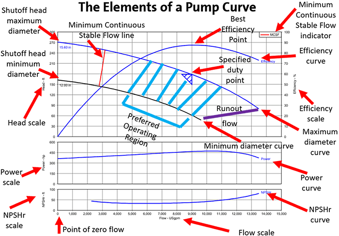 Image 1. Single speed curve (Images courtesy of Grundfos)
To illustrate, consider the following example and refer to the single speed curve displayed in Image 1:
- a flow of 9,000 gpm
- a head of 180 feet
Locate 9,000 gpm on the x-axis, and follow it up until it intersects with 180 feet of head on the y-axis. The intersection point would fall toward the middle of the curve and likely be within the POR, making the pump a good choice for this example application.
It would be important to confirm that it does in fact fall within the POR by checking the manufacturer’s guidelines.
The same graph can represent how the pump’s performance will change if the impeller diameter is reduced or enlarged. The diameter is expressed in inches neighboring its respective curve. A change in impeller diameter does not affect the system curve, which only shifts if there is a change in system head, such as a closed valve. The intersection points are where the pump will perform at each diameter.
Note that it is permissible to change the impeller diameter, as well as system conditions, so long as the pump performance still falls within the POR. There is a broader range of the pump curve identified as the allowed operating region (AOR), in which it may be permitted and beneficial to operate the pump. It normally falls between the minimum continuous stable flow (MCSF) line and the runout line. If pump performance falls outside that zone, look for another pump.
Other Pump Curve Elements
In addition to plotting the pump and system curves, a pump curve graph provides other elements important for choosing the correct product for your application.
Efficiency curve: The pump efficiency curve represents a pump’s efficiency across its entire operating range. Efficiency is expressed in percentages on the right of the curve graph. The BEP is represented by the efficiency curve’s peak, with efficiency declining as the curve arcs away, either right or left, from the BEP. Knowing the efficiency percentage will also help calculate horsepower required for an application.
ISO efficiency lines: International Organization for Standardization (ISO) lines are concentrically elliptical curves indicating equal efficiency on a pump curve graph. They are used as another means of representing how efficiency levels change along a pump curve as it moves away from the BEP or if the impeller diameter is reduced.
Power curve: The power curve represents the load the pump imposes on the driver at a given point on the pump curve and helps with proper motor sizing. It is represented as a separate curve graph and gradually rises toward its peak load, which is typically close to the BEP with most rotodynamic pump types. Afterward, it declines as it approaches the runout point.
Net positive suction head curve: The net positive suction head required (NPSHr) indicates how much force is needed to push liquid into the eye of the pump impeller. It is displayed in feet beneath the main pump curve graph. Knowing the correct amount of NPSHr will prevent the pump from cavitating, vibrating and failing prematurely.
Variable Speed Pumps
Thus far, only fixed, single-speed pumps have been considered. Now let us take a brief look at the variable speed curve, shown in Image 2.
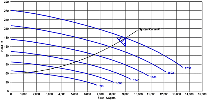 Image 2. Variable speed curve
When noted on the graph, the various speeds are represented in rpm by separate curves. As the speed is reduced, the variable speed pump curves help predict what the corresponding reductions will be to flow and head levels, based on their intersection points with the system curve. Along the system curve arc, the reductions continue until the flow and head eventually reach zero and the pump rpm stops. Additional system curves can also be added to illustrate, for example, the impact of various zone valves opening and closing as in a heating, ventilation and air conditioning (HVAC) system. Note that depending on the type of speed control used, the pump may operate on a control curve that is different than the system curve.
The above terms and considerations cannot cover every scenario a specifier may encounter. However, understanding them will help provide a solid foundation for interpreting a pump curve.
This, in turn, will foster sound decisions when selecting and specifying pumps.
Editor’s note: In 2016, Grundfos and Pumps & Systems presented a webinar on a similar topic to this article. Attendees found it very useful, and we believe readers of this article may also find it helpful to build on the knowledge they gained. To learn more about how to read a pump curve, you can download an archived version of the webinar here.